Visualising imaging data

RamanSPy allows the visualisation of Raman imaging data. Visualising imaging data can be achieved by utilising the ramanspy.plot.image() or ramanspy.SpectralImage.plot() method.

To show how that can be done, in this example, we will use the Volumetric cell data provided in RamanSPy. Below, we load the volumetric data across a cell and select a particular layer from the volume (here, this is the fourth layer).

import ramanspy
dir_ = r'../../../../data/kallepitis_data'

volumes = ramanspy.datasets.volumetric_cells(cell_type='THP-1', folder=dir_)

cell_layer = volumes[0].layer(4)  # only selecting the fourth layer of the volume

Having loaded a ramanspy.SpectralImage object, we can directly plot a spectral slice across a specific band of the image using its ramanspy.plot.image() method. Here, this is the 1008 cm :sup: -1 band.

ramanspy.plot.image(cell_layer.band(1008))

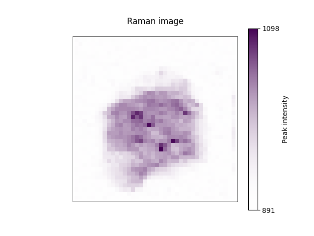
<Axes: title={'center': 'Raman image'}>

We can achieve the same behaviour using the ramanspy.SpectralImage.plot() method, too.

cell_layer.plot(bands=[1008])

<Axes: title={'center': 'Raman image'}>

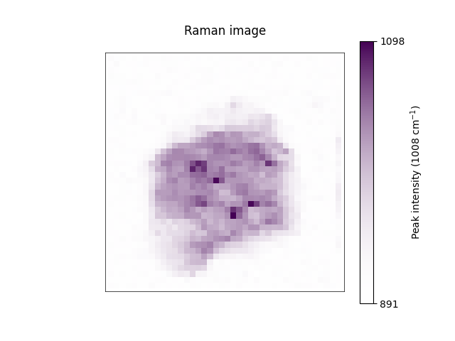
As usual, RamanSPy provides a broad control over the characteristics of the plot. For instance, we can add more informative title, axis labels, colorbar label, colour schemes, etc.

ramanspy.plot.image(cell_layer.band(1008), title="Cell imaged with Raman spectroscopy", cbar_label=f"Peak intensity at 1008cm$^{{{-1}}}$")

<Axes: title={'center': 'Cell imaged with Raman spectroscopy'}>

Users can also use RamanSPy to save the image to a file.

ax = ramanspy.plot.image(cell_layer.band(1008))
ax.figure.savefig("cell_image.png")

It is also possible to plot several images at the same time. When doing that, separate plots will be produced.

cell_layer.plot(bands=[1600, 1008])

# or ramanspy.plot.image([cell_layer.band(1600), cell_layer.band(1008)])

• 
• 

[<Axes: title={'center': 'Raman image'}>, <Axes: title={'center': 'Raman image'}>]

Check the rest of the documentations of the two functions for more information of the available parameters.