Preprocessing pipelines

In this example, we will see how easy it is to construct, customise and reuse preprocessing protocols with RamanSPy.

Data used is from [1].

Prerequisites

import matplotlib.pyplot as plt
import random
import numpy as np

import ramanspy

Set random seed for reproducibility

random.seed(42)

Define color palette.

colors = plt.cm.get_cmap()(np.linspace(0, 1, 4))

Set up global figure size.

plt.rcParams['figure.figsize'] = [4, 2]

Data loading

Loading the data.

thp1_volumes = ramanspy.datasets.volumetric_cells(cell_type='THP-1', folder=r'../../../data/kallepitis_data')

# selecting the first volume
thp1_volume = thp1_volumes[0]

Grab 2 random spectra from the volume

random_spectra_indices = random.sample(range(thp1_volume.flat.shape[0]), 2)
random_spectra = list(thp1_volume.flat[random_spectra_indices])

Plot the raw spectra

_ = ramanspy.plot.spectra(random_spectra, color=colors[1], plot_type='separate')

• 
• 

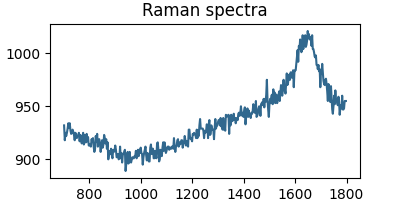
Plot the fingerprint region

cropper = ramanspy.preprocessing.misc.Cropper(region=(700, 1800))
fingerprint_region = cropper.apply(random_spectra)
_ = ramanspy.plot.spectra(fingerprint_region, color=colors[1], plot_type='separate')

• 
• 

Pipelines

Below, we will investigate a series of preprocessing pipelines and their effect on the spectra.

Pipeline I

Applying a preprocessing protocol which consists of:

• spectral cropping to the fingerprint region (700-1800 cm-1);

• cosmic ray removal with Whitaker-Hayes algorithm;

• denoising with a Gaussian filter;

• baseline correction with Asymmetric Least Squares;

• Area under the curve normalisation (pixelwise).

Define the pipeline

pipe = ramanspy.preprocessing.Pipeline([
    cropper,
    ramanspy.preprocessing.despike.WhitakerHayes(),
    ramanspy.preprocessing.denoise.Gaussian(),
    ramanspy.preprocessing.baseline.ASLS(),
    ramanspy.preprocessing.normalise.AUC(pixelwise=True),
])

# preprocess the spectra
preprocessed_spectra = pipe.apply(random_spectra)

# plot the results
_ = ramanspy.plot.spectra(preprocessed_spectra, color=colors[3], plot_type='separate')

• 
• 

Pipeline II

Applying a preprocessing protocol which consists of:

• spectral cropping to the fingerprint region (700-1800 cm-1);

• cosmic ray removal with Whitaker-Hayes algorithm;

• denoising with Savitzky-Golay filter with window length 9 and polynomial order 3;

• baseline correction with Adaptive Smoothness Penalized Least Squares (asPLS);

• MinMax normalisation (pixelwise).

# preprocess the spectra
pipe = ramanspy.preprocessing.protocols.Pipeline([
    cropper,
    ramanspy.preprocessing.despike.WhitakerHayes(),
    ramanspy.preprocessing.denoise.SavGol(window_length=9, polyorder=3),
    ramanspy.preprocessing.baseline.ASPLS(),
    ramanspy.preprocessing.normalise.MinMax(pixelwise=True),
])
preprocessed_spectra = pipe.apply(random_spectra)

# plot the results
_ = ramanspy.plot.spectra(preprocessed_spectra, color=colors[0], plot_type='separate')

• 
• 

Pipeline III

Applying a preprocessing protocol inspired from [2] which consists of:

• spectral cropping to the fingerprint region (700-1800 cm-1);

• cosmic ray removal with Whitaker-Hayes algorithm.

• baseline correction with polynomial fitting of order 2;

• (Unit) Vector normalisation (pixelwise).

# preprocess the spectra
pipe = ramanspy.preprocessing.Pipeline([
    cropper,
    ramanspy.preprocessing.despike.WhitakerHayes(),
    ramanspy.preprocessing.baseline.Poly(poly_order=3),
    ramanspy.preprocessing.normalise.Vector(pixelwise=True)
])
preprocessed_spectra = pipe.apply(random_spectra)

# plot the results
_ = ramanspy.plot.spectra(preprocessed_spectra, color=colors[2], plot_type='separate')

• 
• 

References

[1]

Kallepitis, C., Bergholt, M., Mazo, M. et al. Quantitative volumetric Raman imaging of three dimensional cell cultures. Nat Commun 8, 14843 (2017).

[2]

Bergholt MS, St-Pierre JP, Offeddu GS, Parmar PA, Albro MB, Puetzer JL, Oyen ML, Stevens MM. Raman spectroscopy reveals new insights into the zonal organization of native and tissue-engineered articular cartilage. ACS central science. 2016 Dec 28;2(12):885-95.